hictkR Vignette • hictkR

Opening files

hictkR supports opening .hic and .cool files using the File() function.

When opening files in .hic format, resolution is a mandatory parameter.

path <- system.file("extdata", "interactions.hic", package="hictkR")
f <- File(path, resolution=100000)

hictkR file handles returned by File() provide several attributes storing static properties of the opened file

path <- f$path
resolution <- as.integer(f$resolution)

paste("File \"",
      basename(path),
      "\" has the following resolution: ",
      resolution,
      "bp",
      sep="")

File “interactions.hic” has the following resolution: 100000 bp

Accessing chromosomes and bins

Some of these properties store the list of chromosomes as well as the bin table associated with the opened file.

chroms <- f$chromosomes
bins <- f$bins
normalizations <- f$normalizations

Chromosomes
name	chr2L	chr2R	chr3L	chr3R	chr4	chrX	chrY	chrM
size	23513712	25286936	28110227	32079331	1348131	23542271	3667352	19524

Bin table
chrom	chr2L	chr2L	chr2L	chr2L	chr2L	chr2L	…
start	0	1e+05	2e+05	3e+05	4e+05	5e+05	…
end	1e+05	2e+05	3e+05	4e+05	5e+05	6e+05	…

Normalizations
ICE

Fetching interactions

hictkR support fetching interactions through the fetch() function.

Fetch genome-wide interactions with genomic coordinates

fetch(f, join=TRUE)

chrom1	end1	chrom2	start2	end2	count
chr2L	100000	chr2L	0	100000	101360
chr2L	100000	chr2L	100000	200000	29915
chr2L	100000	chr2L	200000	300000	4996
chr2L	100000	chr2L	300000	400000	2252
chr2L	100000	chr2L	400000	500000	3705
chr2L	100000	chr2L	500000	600000	2446

Interactions can also be normalized using one of the available normalization methods (see f$normalizations).

fetch(f, join=TRUE, normalization="ICE")

chrom1	end1	chrom2	start2	end2	count
chr2L	100000	chr2L	0	100000	0.6915117
chr2L	100000	chr2L	100000	200000	0.1748966
chr2L	100000	chr2L	200000	300000	0.0373811
chr2L	100000	chr2L	300000	400000	0.0238225
chr2L	100000	chr2L	400000	500000	0.0194293
chr2L	100000	chr2L	500000	600000	0.0158976

Fetch interactions for a region of interest

hictkR can be instructed to fetch interactions for a region of interest.

This is much more efficient than fetching genome-wide interactions and then filtering interactions using R.

fetch(f, "chr2L", join=TRUE)

chrom1	end1	chrom2	start2	end2	count
chr2L	100000	chr2L	0	100000	101360
chr2L	100000	chr2L	100000	200000	29915
chr2L	100000	chr2L	200000	300000	4996
chr2L	100000	chr2L	300000	400000	2252
chr2L	100000	chr2L	400000	500000	3705
chr2L	100000	chr2L	500000	600000	2446

fetch(f,
      "chr2L:0-10,000,000",
      "chr3R:10,000,000-20,000,000",
      join=TRUE)

chrom1	end1	chrom2	start2	end2	count
chr2L	100000	chr3R	10000000	10100000	55
chr2L	100000	chr3R	10100000	10200000	52
chr2L	100000	chr3R	10200000	10300000	26
chr2L	100000	chr3R	10300000	10400000	31
chr2L	100000	chr3R	10400000	10500000	22
chr2L	100000	chr3R	10500000	10600000	22

Fetch interactions as a dense matrix

hictkR can return interactions as a Matrix when specifying type="dense".

fetch(f,
      "chr2L:0-1,000,000",
      "chr3R:1,000,000-2,000,000",
      type="dense")
#>       [,1] [,2] [,3] [,4] [,5] [,6] [,7] [,8] [,9] [,10]
#>  [1,]   11    4    9    7   10    1   15    3    5    29
#>  [2,]   11   10   15    4   14    7    5    2   12    44
#>  [3,]    6    5   11    8   12    8    6    3   12    30
#>  [4,]    6    2    8    3    5    7    1    2    7    15
#>  [5,]    9    9   12   11   18   12    9    2   11    46
#>  [6,]   17    7   13    4   16    8    1    4    9    64
#>  [7,]    2    2    4    4    5    5    5    0    8    20
#>  [8,]    3    6   11    4   11    7    3    1    9    19
#>  [9,]   17    6    7    4   11    9    3    1   14    76
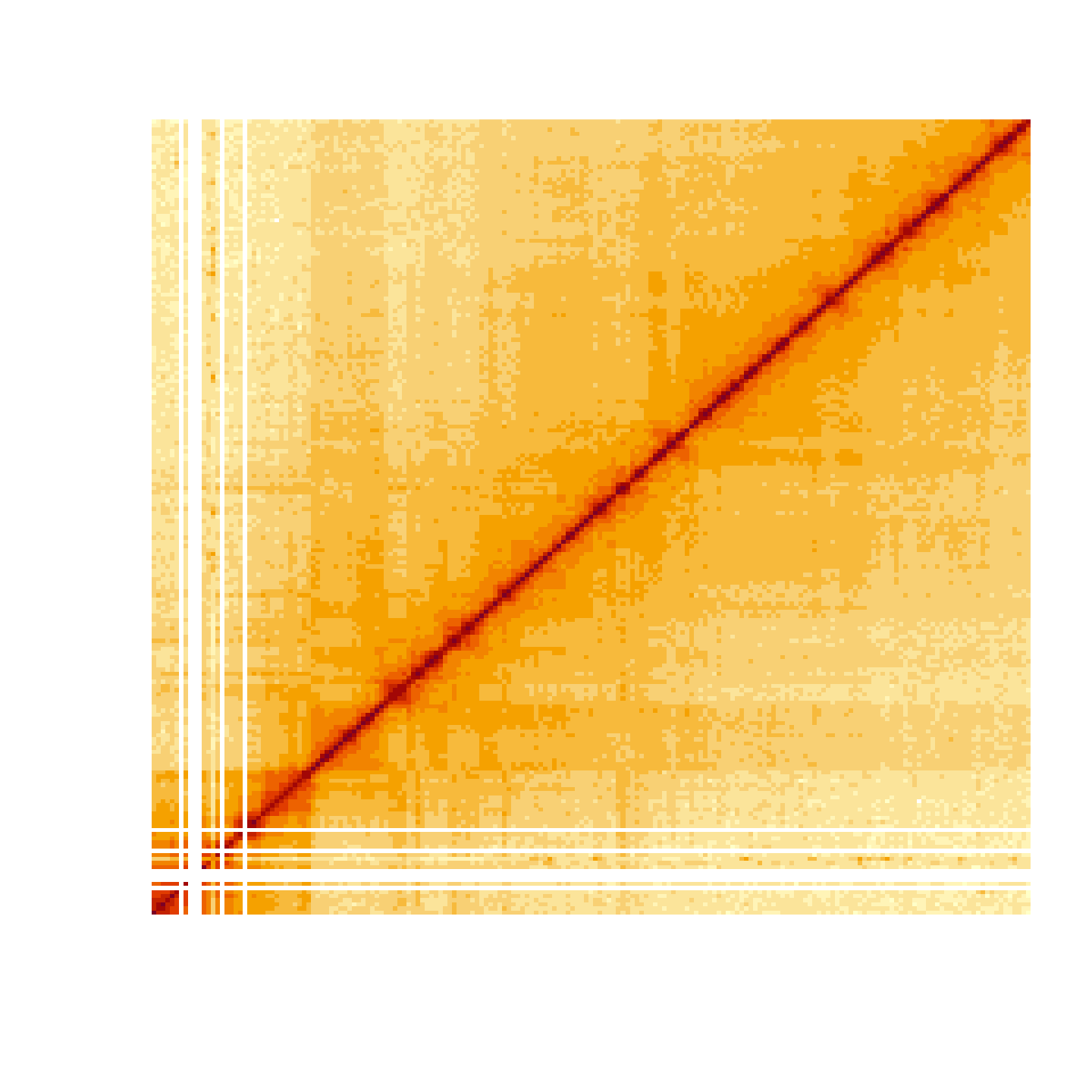
#> [10,]    0    2    9    2    7    2    4    1    3     7

This can be very useful to visualize interaction matrices as heatmaps.

m <- fetch(f, "chr3R:0-20,000,000", normalization="ICE", type="dense")
image(log(m), axes=FALSE)